The integration of BI solutions within business process applications or interfaces has become a modern standard. Over the past two decades, Business Intelligence has dramatically transformed how data could be used to drive business and how business processes can be optimized and automated by data. With ML and augmented analytics movement, BI applications are vital to every organization. Analytics embedding enables capabilities such as interactive dashboards, reporting, predictive analytics, AI processing and more within the touch of existing business applications. This differs from traditional standalone BI applications that put all the capabilities of business intelligence directly within the applications on which users have already relied. Now you may ask, when should I consider embedding to maximize my ROI?

Embedding Use Cases

Bar graph with upward trend     Business Process Applications

In this case, the integration of data & analytics is embedded into applications used by specific personas. For instance, embedding historical client information into a CSR application. One outcome will be improved decision-making based on readily available customer insights and higher levels of user adoption.

Shopping cart    Software / OEM Solutions

Digital transformation is all about software. Data visualization, forecasting and user interactions are must-have features of every application. Save the time you would spend coding. Embedding analytics in software not only saves cost greatly but also prominently enhances functionalities of software application.

Forest scene     Portals / Websites

Integration of data into your website or portal is another popular option. The benefits are obvious – information sharing provides your customers with valuable insights through a unified platform; you are able to go to market much faster since you are reaching customers directly. It helps your customers access the data they need to make decisions better, quicker and within their fingertips.

Embedding flow for embedding for your customers

Prepare for Embedding

Ready to get started? Let’s take a look at things to be considered. At a high level, the following areas to be carefully examined before design begins:

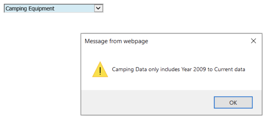
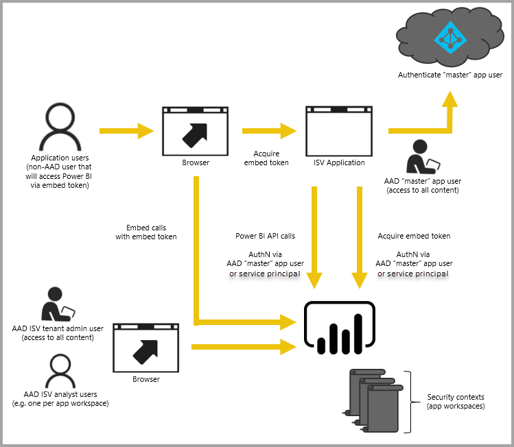
  • What are the embedding integration options? Especially with regards to security, how do you enable other application access to your secured BI assets? What are the options to manage authentication and authorization for thousands of users, both internally and externally?
  • Which functionalities will be open and accessible to BI embedding specifically? Typically not all UI functionalities are supported via embedding. Verify that critical functionalities are supported. Map your requirements to embedding functionalities and features.
  • Cloud vs On-premise hosting. Besides management and cost concerns, your organization may have cloud strategies and road-maps in place already. If that is the case, most likely no exception for BI application including embedding. Plus source data cloud modernization is another big driver to go with cloud. 
  • Cost – yes, no surprise there is cost associated with BI embedding. Each BI vendor may collect fees differently but legitimately you will need to pay BI embedding based on consumption pattern even when a single application user account is leveraged. Do the math so you know how much it will be on the bill. 

 Next let’s examine the tool differences. 

Embedding API by Leading BI Vendors

VendorAPIFunctionalities
IBM CognosSDK – Java, .NetMashup Service (Restful)New JavaScript API for DashboardNew REST API   Full programming SDK is almost identical to UI functionalitiesSDK can execute or modify a reportMashup service is easy to web embedding, limited report output formats are supportedJavaScript API and extension for dashboard, display/editNew REST API for administration 
Power BIREST APIJavaScriptREST: Administration tasks, though clone, delete, update reports are supported tooJavaScript: provides bidirectional communication between reports and your application. Most embedding operations such as dynamic filtering, page navigation, show/hide objects 
TableauREST APIJavaScriptREST: manage and change Tableau Server resources programmaticallyJavaScript: provides bidirectional communication between reports and your application. Most embedding operations such as dynamic filtering, page navigation
AWS QuickSightSDK – Java, .Net, Python, C++, GO, PHP, Ruby, Command lineJavaScriptSDK  to run on server side to generate authorization code attached with dashboard urlJavaScript: parameters (dynamic filters), size, navigation

BI embedding opens another door to continue serving and expanding your business. It empowers business users to access data and execute perceptive analysis within the application they are familiar with. Major BI vendors have provided rich and easy to use API, the development effort is minimum, light and manageable while the return benefits are enormous. Have you decided to implement BI Embedding yet? Please feel free to contact Ironside’s seasoned BI embedding experts to ask any questions you may have. We build unique solutions to fit distinctive requests, so no two projects are the same, but our approach is always the same and we are here to help.

For users of IBM Cognos Analytics a popular request is to highlight alternating rows in a report. This article will demonstrate how to achieve this result using the list container and the property Conditional Styles.

In order to create the report, the following objects will be used:

Object Definition
List containerContains report data
Query CalculationsCreate calculations
Running-count() functionGet sequential numbers
Mod() functionGet remainders of 0 or 1
List columns body style ancestorAncestor object used to highlight the data
Conditional stylesCreate type of style

Finished Product

When the demo is finished your report will look similar to the following:

Let’s get started.  The first thing we’ll do is create a simple list report using the sample GO Sales (query) package included with the application.  However, you can use any data to follow along.  

Create the query calculation

  1. Select the blank template and create a report using the List container. 
  2. From the Sales(query) namespace add the Product number, Product and Revenue data items to the list.
  1. View the report in Page Preview.
  1. From the Toolbox, add a Query Calculation to the end of the list container next to Revenue.  The Data item expression dialog will open. Name the calculation Count
  2. Click the Functions tab at the bottom of the screen.   
  1. Open the Summaries folder and double click the running-count() function to add it to the expression.  This function returns the running count by row for a set of values.
  1. Click the second tab on the dialog box, Data Items , and drag the Product Number to the function.  Add the ending parenthesis.

Running-count(Product number)

  1. Click OK to view the results.

The result of the running-count() function will show sequential numbers on each row.

Create Values to Highlight

The mod() function returns the remainder of two numbers.  In our case it will generate the numbers 0 or 1 after the division takes place.  

We will nest the mod() function around the running-count() function to achieve this result.

  1. Double-click the Count column title to return to the Data item expression.
  2. Modify the expression as follows.

mod(running-count([Product number),2)

  1. Click OK when done to view the report.  Note the position of the parentheses and the divisor is 2.  Even numbers will have a remainder of 0 and odd 1.

Note:  the mod()function is available for selection, however, we are typing the expression to ensure the correct syntax is applied.

The results of the calculation show 0 and 1 on alternating rows. 

 Apply Conditional Formatting

We will now highlight the rows in the list object using the List Columns Body Style ancestor. A row with the value of 1 will be colored.

  1. Click any column in the List container and at the top of the Properties pane or on the flyout menu select the ancestor object and click List Columns Body Style.  When selected the area will highlight in the list.

2.  From the Properties pane double click the Conditional Styles property.  The Conditional Styles dialog box will appear.  Click the plus sign (+) and select New Conditional style > Count. Click OK.

  1. Click the plus sign (+) to add a threshold value of 0 and click OK.  In the Style column click the first edit button (pencil) and select a Background color. Click OK.  Note the arrow next to the 0 is pointing upward indicating the color will generate for values greater than 0. Click OK to exit all dialog boxes.
  1. View the report.

5.  Since the Count column is not needed in the report remove it using the Cut button (scissors). Do not delete the column as it is used in the calculation used to render the conditional formatting and must remain in the underlying query.

As you can see, alternating row colors in a list report is simple in IBM Cognos Analytics!

Happy reporting! 

For the original version of this blog post using IBM Cognos Workspace Advanced, click here.

Determinants can play a crucial role in the overall performance and consistency of your Framework Manager model but remain one of the most confusing aspects of the application to most developers. This article will attempt to end the confusion.

Determinants are used so that a table of one grain (level of detail) behaves as if it were another actually stored at another grain. They are primarily used for dimension tables where fact tables join to dimension tables at more than one level in the dimension. (There are other cases where you could use them, but they are less common and fairly specific situations.)

The Situation

Let’s use the example of a date dimension table with day level grain. If all the fact tables join at the day level, the most detailed level, then you do not need determinants.  But as many of us know from experience, this is not always the case. Fact table are often aggregated or stored at different levels of granularity from a number of reasons.

The Problem

The trouble arises when you wish to join to the dimension table at a level that is not the lowest level. Consider a monthly forecast fact table which is at the month level of detail (1 row per month). A join to the month_id (e.g. 2009-12) would return 28 to 31 records (depending on the month) from the date dimension, and throw off the calculations. Determinants solve this problem.

The SQL

Often when modeling, it’s useful to think about the SQL code you would like to generate. Without determinants, the incorrect SQL code would look something like this.

SELECT
F.FORCAST_VALUE,
D.MONTH_ID,
D.MONTH_NAME
FROM SALES_FORECAST F INNER JOIN DATE_DIM D ON
F.MONTH_ID = D.MONTH_ID

This code will retrieve up to 31 records for each of the sales forecast records. Applying mathematical functions, for example Sum and Count, would produce an incorrect result. What you would like to generate is something along the following lines, which creates a single row per month, AND THEN join to the fact table.

SELECT
F.FORCAST_VALUE,
D1.MONTH_ID,
D1.MONTH_NAME
FROM SALES_FORECAST F INNER JOIN
( SELECT DISTINCT
D.MONTH_ID,
D.MONTH_NAME
FROM DATE_DIM D ) AS D1
ON F.MONTH_ID = D1.MONTH_ID

As shown  above, the trick is to understand which columns in the dimension table are related to the month_id, and therefore are unique along with the key value.  This is exactly what determinants do for you.

Unraveling the Mystery in Framework Manager

Following Cognos best practices, determinants should be specified at the layer in the model in which the joins are specified.

Here we see a date dimension with 4 levels in the dimension, Year, Quarter, Month and day level.

This means we can have up to 4 determinants defined in the query subject depending on the granularity of the fact tables present in your model.  The first three levels, Year, Quarter, Month, should be set to “group-by” as they do not define a unique row within the table and Framework Manager needs to be made aware that the values will need to be “Grouped” to this level. In other words, the SQL needs to “group by” a column or columns in order to uniquely identify a row for that level of detail (such as Month or Year).  The Day level (often called the leaf level) should be set to “Uniquely Identified”, as it does uniquely identify any row within the dimensional table. While there can be several levels of “group by” determinants, there is typically only one uniquely identified determinant, identified by the unique key of the table. The “uniquely identified” determinant by definition contains all the non-key columns as attributes, and is automatically set at table import time, if it can be determined.

The Key section identifies the column or columns which uniquely identify a level.  Ideally, this is one column, but in some cases may actually need to include more than one column.  For example, if your Year and Month values (1-12) are in separate columns.  In short, the key is whatever columns are necessary to uniquely identify that level.

Using our aforementioned table, the setup would look like this:

The Attributes section identifies all the other columns which are distinct at that level.  For example, at a month_id  (e.g. 2009-12) level , columns such as month name, month starting date, number of days in a month are all distinct at that level. And obviously items from a lower level, such as date or day-of-week, are not included at that level.

Technically, the order of the determinants does not imply levels in the dimension. However, columns used in a query are matched from the top down which can be very important to understanding the SQL that will be generated for your report. If your report uses Year, Quarter and Month, the query will group by the columns making up the Year-key, Quarter-key and Month-key. But if the report uses just Year and Month (and not the Quarter) then the group by will omit the Quarter-key.

How Many Levels Are Needed?

Do we need all 4 levels of determinants? Keep in mind that determinants are used to join to dimensions at levels higher than the leaf level of the dimension. In this case, we’re joining at the month level (via month_id). Unless there are additional joins at the year or quarter level, we do not strictly need to specify those determinants. Remember that year and quarter are uniquely defined by the month_id as well, and so should be included as attributes related to the month, as shown.

The Result

Following these simple steps the following SQL will be generated for your report. The highlighted section is generated by the determinant settings. Notice how it groups by the Month_ID, and uses the min function to guarantee uniqueness at that level.  (No, it doesn’t trust you enough to simply do a SELECT DISTINCT.)  The second level of group by is the normal report aggregation by report row.  So the result is that the join is done correctly, which each monthly fact record joined to 1 dimensional record at the appropriate level, to produce the correct values in the report.

This blog is an updated version of a previously released post, which can be found here.

Gathering data is an essential step before performing analysis in Power BI Desktop. The tool allows users to connect with many different data sources, such as traditional or cloud databases, text files, big data, and live streams. Among these sources are SQL Server Analysis Services (SSAS) Tabular models, which are widely leveraged for enterprise solutions. Why? Let’s dive into Tabular Modeling to learn more.

Read more

In the first installment of this series, we discussed the origins of Mode 2 Analytics, and in the second installment we focused on how to enable this capability in your organization using Cognos. Now that we’ve learned all about how Mode 2 works, let’s walk through a sample use case that highlights the Bimodal Analytics Lifecycle as well as the technical capabilities of Cognos Analytics and how they fit together.

In this example, you are the manager of a Healthcare Call Center system that is comprised of seven (7) regional centers across the country. Each call center handles contact (phone calls and online chats) from the customers that are located within the states that make up those regions.

Read more

What is the most common, most vital need of any business? Speed.

Speed to adapt, to respond, to evolve. It is important, not just at the big picture level, but on a daily basis as well. If you’re constantly waiting for information, then you’re spending less time analyzing data and making decisions that help the organization. Speed has been vitally important in the acceptance of Mode 2 style content such as Dashboards and Stories. Response time is key when viewing daily high-level metrics or when creating that “single use” asset to analyze a potential issue.

Read more

In previous releases of Cognos Analytics, we have seen a trend of integrating many of the features of metadata modeling in Framework Manager into the Cognos Analytics interface. This trend is continuing with new or improved modeling capabilities being incorporated into Cognos Analytics 11.1 Data Modules.

Read more

With the maturing and ever increasing acceptance of the cloud across multiple industries and the data gravity gradually moving to the cloud, i.e. more data being generated in the cloud, we are seeing some interesting cloud-based data and analytics platforms offering unique capabilities. Some of these platforms could be disruptive to the established market leaders with their innovative thinking and ground up design that is “born in the cloud and for the cloud.”

Read more

In the first installment of our series on bimodal analytics, we talked about the origins of Mode 2 analytics. We looked at some of the challenges around implementing true bimodal analytics within IBM Cognos Analytics 11 and touched on some of the vendors who were born as Mode 2 platforms. This second installment will focus specifically on how to enable Mode 2 analytics within the organization using Cognos.

Read more