Recipes for Predictive Modeling: Highly Imbalanced Data

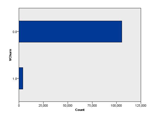
Suppose you’re trying to build a model to predict respondents, and in your data set, about 3% of the population will respond (target = 1). Without applying any specific analysis techniques, your prediction results will likely be that every record is predicted as a non responder (predicted target = 0), making the prediction result insufficiently informative. This is due to the nature of this kind of information, which we call highly imbalanced data.
The imbalanced nature of the data can be intrinsic, meaning the imbalance is a direct result of the nature of the data space , or extrinsic, meaning the imbalance is caused by factors outside of the data’s inherent nature, such as data collection, data transportation, etc.
As data scientists, we’re mostly interested in intrinsic data imbalance; more specifically, the relative imbalance of a data set. In this case, the absolute number of the positive cases (the 1s) may not be small, but the corresponding number of negative cases (the 0s) is much larger, ensuring that there are always far more negative cases than positive ones.
Intrinsic imbalance doesn’t necessarily lead to low effectiveness of standard learning algorithms. There may be one or more predictors highly correlated with the target results. Therefore, poor effectiveness of learning results on highly imbalanced data is usually caused by a combination of weak predictors, data, domain complexity, and data imbalance. For example, the predictors used might not produce strong correlations with the target variable, causing the negative cases to constitute up to 97% of all the records. In this case, the learning algorithm will try to make a best guess, and if the predictors don’t provide enough information it will just guess a negative/non respondent/zero value as this is much more likely to happen overall.
Note: The description above makes it sound like highly imbalanced data can only occur with binary target variables, which is not true. Nominal target variables can also suffer from the problem of high imbalance. This article, however, only illustrates with the more common binary imbalance example.
Luckily, there are a lot of research options that mitigate the problem of poor learning algorithm performance on highly imbalanced data. Most of the developed methodologies work on the following four aspects of the data: training set size, class prior, cost matrix, and placement of decision boundary . By leveraging SPSS Modeler’s functional expandability through its integration with R, you can deploy the majority of these developed techniques, if not all of them. We’ll focus on exploring the methods that can be directly implemented with SPSS Modeler itself in this article.
Training Set Size Manipulation (Sampling Methods)
Intuitively, many data scientists will think of undersampling and oversampling as a possible solution, which would mean either randomly taking out some major class records (records belonging to the target class of majority) or randomly selecting some minor class records and appending them to the whole data set. Both approaches can succeed in balancing out the classes, and many complicated methods have been developed based on this simple initial instinct.
The most straightforward of these methods is of course random oversampling and undersampling. With random oversampling, however, no new information is added to the dataset but rather a number of minor class records are duplicated. As some of the otherwise non-predictive features get repeated and accentuated through random oversampling, you may end up in an overfitting situation where statistically irrelevant factors suddenly appear to have an impact. This problem is a double-edged sword, though, because undersampling can lead to the opposite problem of skipping some potentially useful information.
A lot of approaches have been developed to improve the balance of the data and maintain the information accuracy of the data during random sampling. We’ll discuss the EasyEnsemble and BalanceCascade methods in detail here.
Random Oversampling and Undersampling
One simple way to rebalance data in SPSS Modeler is with a Balance node. This node carries out simple random oversampling by assigning a factor larger than 1 to the minority class. It can also perform simple random undersampling by assigning a factor smaller than 1 to the majority class.
EasyEnsemble
The idea behind EasyEnsemble is very simple. Several subsets of samples are created independently from the major class cases of the original dataset. Each subset of the major class cases should be about the same size as the minor class. Each time, a subset of the majority class records gets selected and appended to all the minority class records. Then, you train a classifier on this appended subset of data. This process is reiterated multiple times until all the subsets of the majority class are modeled. In the end, you combine all the classifiers created to produce final classification results.
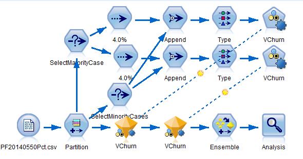
We’re going to show you an implementation of this method with SPSS Modeler.
To begin, connect a Sample node with the upper stream Select node, selecting all the majority class cases and make sure to deselect the Repeatable partition assignment option so you can make sure sure that the every subset of the sample is created independently. Append the sample with the minority class cases. Run the modeling node on the appended data. Repeat this with multiple Sample nodes.
BalanceCascade
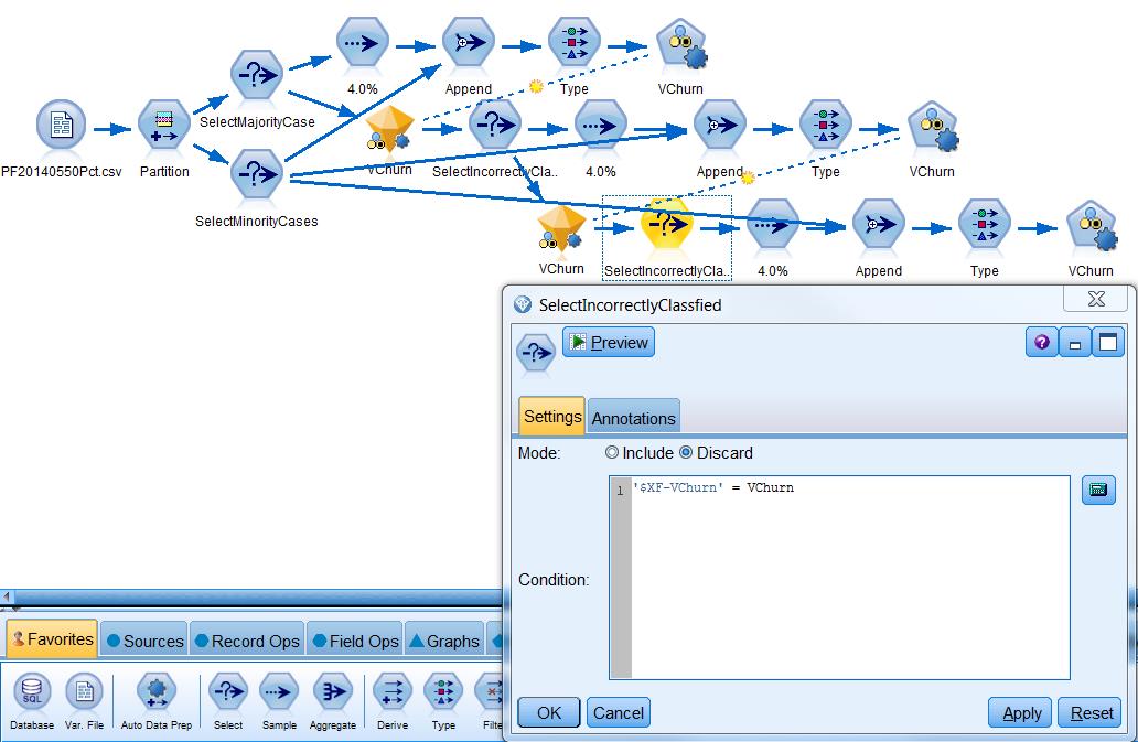
BalanceCascade takes a more supervised approach to undersampling. You start this method by constructing a subset made up of all the minority cases and a random sample of the majority class that is about the same size as the minority class. After training on this subset, you take out the majority cases that can be classified correctly by the trained classifier and use the rest of the majority cases to go through the process again until the number of majority cases left is smaller than that of the minority cases. In the end, you combine the classifiers of all these iterations in such a way that only the cases classified as responder/positive by all the classifiers will be marked as responder/positive.
It’s a little trickier to implement this method in SPSS Modeler. There are probably multiple ways of doing this, and here we’ll just show one of them that reiterates the process once. You begin with randomly sampling from the major class cases again. Next, you use the Auto Classifier node to build a preliminary model off of the appended subset. After that, you need to score all the major class cases with it and discard those correctly classified major class cases with a Select node.
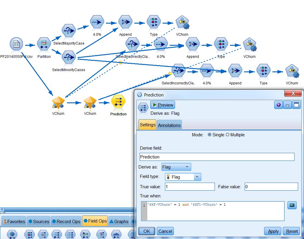
When deploying the model nuggets that get generated during this process, you need to connect all of them to the data source and derive a rule similar to the one shown below.
Cost Matrix Manipulation
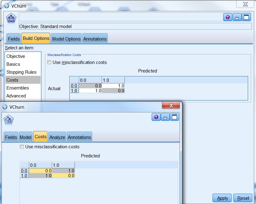
While sampling methodologies try to alter the distributions of different classes, cost matrix manipulation alter the misclassification penalty. Usually, misclassifying a majority class as a minority class incurs a smaller cost than misclassifying a minority class as a majority class. For example, when trying to identify cancer patients with their mammography exams, one would expect that misclassifying a cancer patient as a non-cancer patient is far more costly than the other way around.
SPSS makes it pretty easy to implement misclassification cost manipulation. In a modeling node, you can select the Use misclassification cost option and try out different costs.
Bringing in Class Prior
There are two easy ways of bringing class prior values into your analysis. McCormick et al. introduced a very straightforward approach in 2013 that is a viable option. You can simply compare the propensity score with class prior probability. If the propensity score is larger than the prior probability, you assign the target a new class label marked as positive. An Aggregate node can be used to derive the class prior field. If a raw propensity score is not available, you can use the confidence score, which is the raw propensity score if the target is predicted to be 1 and the raw propensity score minus one if the target is predicted to be 0.
Tim Manns developed another technique for bringing in class prior. Essentially, he proposed to make target variable a continuous variable over the range of 0 and 1 and compare the predicted value with the class prior.
Evaluation of Bringing in Class Prior
It’s worth mentioning that the popular metrics like overall accuracy wouldn’t work in this case. If every record is predicted to be 0, the accuracy will be very high; however, in this situation we want to catch those positive cases. We can use AUC (area under the ROC curve) to accomplish this. AUC has proved to be a more reliable performance measure for imbalanced data. .
Next Steps
If you’d like to learn more about highly imbalanced data or any of the other data science methods we can help you implement, visit the Data Science & Advanced Analytics team page on our website or reach out to us directly to start getting predictive with your business.

References
H. He and E. A. Garcia “Learning from Imbalanced Data”, Knowledge and Data Engineering, IEEE Transactions on, vol. 21, no. 9, pp. 1263 – 1284, 2009
G.M. Weiss, “Mining with Rarity: A Unifying Framework,” ACM SIGKDD Explorations Newsletter, vol. 6, no. 1, pp. 7-19, 2004.
L. Breiman, J. Friedman, R. A. Olshen and C. J. Stone, Classification and Regression Trees. CRC Press, 1984.
X. Liu, J. Wu and Z. Zhou, “Exploratory Undersampling for Class-Imbalance Learning”, Systems, Man, and Cybernetics, Part B: Cybernetics, IEEE Transactions on, vol. 39 , no. 2, pp. 539-550, 2008
K. McCormick, D. Abbott, Meta. S. Brown, T. Khabaza, S. R. Mutchler, IBM SPSS Modeler Cookbook , PACKT Publishing, 2013
T. Manns, 2009, “Building Neural Networks on Unbalanced Data (using Clementine)”, retrieved from http://timmanns.blogspot.com/2009/11/building-neural-networks-on-unbalanced.html
T. Fawcett, “ROC graphs: Notes and practical considerations for researchers”, HP Labs, Tech. Rep. HPL-2003-4, 2003